3. Analysis: what the results mean

Before we start, you have prepared your network, haven’t you? If you haven’t, then go back to Network Preparation. It’s very important.

This section provides an informal introduction to the outputs of sDNA Integral Analysis. Although it focuses or urban networks, the discussion is relevant to all domains of network analysis. A picture speaks a thousand words, so let’s begin with one.

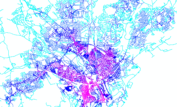
Figure 1: Cardiff link density, 1km radius. Basemap (c) OpenStreetMap contributors

3.1. Links and network radius

The map of Cardiff coloured by link density at 1000m radius shown in Figure 1 makes a good starting point for a discussion about links and radius. This data was output by sDNA Integral with a label of Links R1000, or (in abbreviated format for shapefiles/QGIS) Lnk1000.

Firstly, we have the definition of network link. All links in a spatial network consist of a line joining a junction or dead end, to a junction or a dead end. Junctions and dead ends are the only things that links can join together: any line that doesn’t join two of those things (or one of those things to itself) is not a complete link, though it will certainly be part of a longer line that does join two of those things, and which will therefore be a link.

Note also that links do not connect to junctions except at their endpoints. So in a road network, for example, what you might call a single street will in fact consist of several individual links. A street is defined by its name, a link by geometry alone.

We think link density is a good measure of urban density. The map above is based on a count, for each link, of how many links there are within a 1000m radius around it. Links are the fundamental unit from which spatial networks are built, and for that reason it makes sense to standardize on them as a unit of description. Also, link density tends to hold information about the network. For example, in a road network, link density can correlate over 90% with the density of houses and jobs [1]. Thus link density, in the absence of any other information, gives a pretty good indication of the amount of human activity surrounding any particular point.

[1]	Chiaradia, Alain J., Hillier, Bill, Schwander, Christian and Barnes, Yolande 2013. Compositional and urban form effects on residential property value patterns in Greater London. Proceedings of the ICE - Urban Design and Planning 166 (3) , pp. 176-199. 10.1680/udap.10.00030

The other important thing to discuss in Figure 1 is what the R1000 – the 1000m radius – means. A typical assumption in network analysis is that entities can only travel through the network: cars can’t drive off roads, fish can’t swim through rock, etc. So the 1000m radius is different for each link, and means “all points that can be reached by travelling 1000m through the network from that link”.

For the uninitiated, a network radius is quite hard to visualise. So let’s be clear about this – it’s definitely not a circle. It’s actually a set of link cut points on the network at a variable distance, as the crow flies, from the origin. But some find it easier to visualise a sort of wobbly blob surrounding the origin. Figure 2 illustrates this.

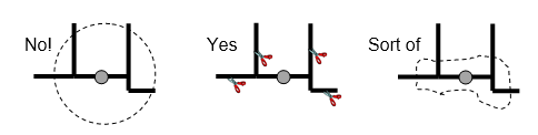
Figure 2: Illustration of what a network radius is, and isn’t.

Lots of output measures from sDNA contain “R1000” - or R followed by a number - as a suffix (in shapefiles/QGIS the R is dropped to save space). These are all radial measures – referring to a specific radial distance (usually expressed in network Euclidean terms, though alternatives are possible). Sometimes output measures contain “Rn”. Radius n means everything: the entire network reachable from the link in question, excluding any parts that aren’t connected.

In continuous space analysis, the radius has a “c” put after it - for example, R500c, R1000c, or Rnc (which as it happens is equivalent to Rn). This shows that the radius is computed using Continuous Space (for more details see Radius). Normally sDNA analysis treats each link as a discrete entity – it is either inside the radius, or it isn’t. Continuous space analysis treats links as continuous entities; if part of the link falls inside the radius, and part outside, then the link is split on-the-fly and we count only the part of that falls inside. Continuous space should always give the most accurate results, but discrete space is faster to compute.

Besides link density, sDNA produces numerous other measures that quantify the network in the radius:

• Total Length is self explanatory
• Number of junctions is self explanatory
• Total Weight is the total weight customizable by the user
• Connectivity is the total number of link ends connected at junctions

3.2. Betweenness

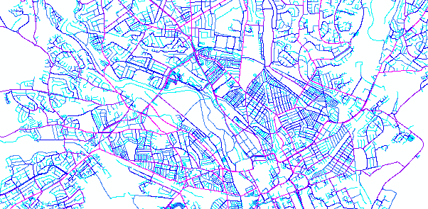
Figure 3: Cardiff Angular Betweenness, Radius 10km. Basemap (c) OpenStreetMap contributors

The flow model inherent in sDNA is based on Betweenness. Figure 3 shows an example. Note this is link-weighted, so the result you see is based on the shape of the network alone.

Betweenness analysis assumes your network is populated with entities that go from everywhere to everywhere else, subject to a maximum trip distance determined by the radius. We assume these entities travel via the shortest possible path – and we call such a path a geodesic. But how we define “shortest” may vary. We call the definition of distance a metric; currently sDNA supports

• Euclidean metrics, taking the shortest physical distance possible
• angular metrics, which minimize the amount of turning both on links and at junctions
• custom metrics based on user data
• other specialist metrics

As a first approach to most urban network problems, we really like using angular metrics. Pedestrians, unless they know an area very well, will tend to follow the shortest angular paths, because they are easier to remember (“second on the right then straight on ‘till morning” – Peter Pan would probably have got lost had he tried to take a short cut requiring more complex directions). Drivers of vehicles also tend to follow angular geodesics, but for a different reason – straight roads through a city tend to be faster, on average. So we have set the default metric in sDNA to be angular.

Take care, however, to set the radius for your intended purpose! A realistic indicator of pedestrian flow might be Betweenness Ang R800, while a realistic indicator of vehicle flow might be Betweenness Ang R2000, or higher. But fish, for example, probably don’t care much about going around corners in rivers, so Euclidean analysis might be more appropriate. Pedestrians commuting to and from work tend to follow Euclidean geodesics too, because they know all the short cuts.

Note that in betweenness analysis, we are usually looking at an intermediate link in a trip, not the origin or destination. This means that the radius has a subtly different meaning: a calculation of betweenness R500 does not involve all possible trips within 500m of the link you are observing, but involves all possible trips that pass through the link you are measuring with a maximum length of 500m (almost: see Geodesic for more details).

A final question in betweenness analysis is what weight to assign to each geodesic. The simplest answer is to assign a weight of 1 to every pair of links. As the density of jobs and homes is strongly related to the density of network links, betweenness weighted in this manner usually correlates well with traffic flows. But what if network length is important to you? Let’s say you want to assume longer streets act as origins and destinations for more people, or you’re analyzing rivers, etc. Or maybe you have custom weights - census data for example, or building entrances. In this case we assume the number of entities making the trip is proportional both to the weight of the origin and the weight of the destination, so we multiply the origin weight and destination weight together to compute the betweenness weight.

Interestingly though, such flows scale with the square of the number of links in the network, implying that more dense areas contain more activity per link - in other words, an opportunity model. (To a physicist, there is a problem with the units: Betweenness is measures in units of weight squared, not weight). If this is not desirable then instead use a Two Phase Betweenness model. These assume each origin has a fixed amount of weight it can add to betweenness – in the case of cities, a fixed quantity of journeys that the people living there will realistically make. This fixed quantity is then divided proportionately among the destination weights accessible from that origin for the current radius; this can be described as a generation-distribution model.

Complementing Two Phase Betweenness is Two Phase Destination – the quantity of visits each destination gets under the two phase model. In the normal betweenness model, each destination will be visited by everything within radius x, so this measure would be equivalent to Weight. But in a two phase model, destinations must compete with other destinations for the attention of origins, and TPDestination measures the total flow to the destination taking account of this competition. A real world example would be the case of high street shops - with small destination weight - trying to compete with an out-of-town retail park - with large destination weight. Both may have lots of population in their catchment (which will show up in the Links Rx measure) but the town centre loses out to the new development (which shows up in the TPDestination Rx measure).

That said, all the forms of betweenness tend to correlate quite well with actual flows of pedestrians, vehicles etc.

3.3. Closeness

Closeness, like betweenness, is a form of network centrality. It matches commonly held notions of accessibility.

Mean Distance is perhaps one of the most common closeness measures in the literature. It measures the difficulty, on average, of navigating to all possible destinations in radius x from each link. Technically then it’s a form of farness not closeness: this only means that big numbers mean “far” instead of “close”.

“Difficulty” is defined in terms of the same metric used for Betweenness: Euclidean, angular, custom, hybrid, and so on. sDNA names its closeness outputs Mean Angular Distance (MAD), Mean Euclidean Distance (MED), Mean Custom Distance (MCD), etc.

Note that the “mean” of mean distance is weighted by the weight of destinations.

3.4. Other measures

sDNA produces numerous other output measures, for a full description refer to Analysis: full specification.

sDNA can also display the geometries of geodesics, network radii and convex hulls used in the analysis, as well as producing accessibility maps for specific origins and destinations.

3.5. Summary of measures

Measure	Abbreviations	Description
Closeness (mean distance)/Farness	MAD, MED, MCD, MHD	Inverse of closeness, accessibility
Mean Geodesic Length	MGLA, MGLE, MGLC, MGLH	As closeness but always output in units of length even for non-Euclidean geodesics
Network Quantity Penalized by Distance	NQPDA, NQPDE, NQPDC, NQPDH	Sum of network quantity over distance
Betweenness	BtA, BtE, BtC, BtH	Flow model, through-movement
Two Phase Betweenness	TPBtA, TPBtE, TPBtC, TPBtH	Generation-distribution flow model
Two Phase Destination	TPDA, TPDE, TPDC, TPDH	Floating catchment, competitive accessibility
Mean Crow Flight	MCF	Mean distance to destinations as crow flies
Diversion Ratio	DivA, DivE, DivC, DivH	Mean ratio of geodesic length to crow flight distance
Convex Hull Area	HullA	Area of convex hull of radius
Convex Hull Perimeter	HullP	Perimiter of convex hull of radius
Convex Hull Max Radius	HullR	Furthest extent of convex hull; crow flight distance for most efficient route
Convex Hull Bearing	HullB	Bearing of furthest extent / most efficient route
Convex Hull Shape Index	HullSI	Describes shape of hull; ranges from 1 for circle to infinity for straight line
Links	Lnk	Links in radius
Length	Len	Length in radius
Weight	Wt	Weight in radius
Angular Distance	AngD	Angularity in radius
Junctions	Jnc	Junctions in radius
Connectivity	Conn	Connectivity in radius
Line Length	LLen	Length of individual polyline
Line Connectivity	LConn	Connectivity of individual polyline
Line Angular Curvature	LAC	Angularity of individual polyline
Line Hybrid Metric	HMf, HMb	Hybrid metric of individual polyline
Line Sinuosity	LSin	Diversion ratio for individual polyline
Line Bearing	LBear	Bearing of individual polyline
Link Fraction	LFrac	Fraction of link represented by polyline

3.6. Calibration

sDNA produces network statistics that correlate to real phenomena such as traffic flows or land prices, but if you are interested in predicting these phenomena, you will need to know how to convert sDNA outputs into a prediction. This is done by regression analysis, a huge topic with which some users of sDNA will already be familiar, but others won’t.

sDNA provides two tools to help with this process, Learn and Predict. Learn takes a sample of real data and creates a model linking it with the output of sDNA. Predict takes a model created by Learn and applies it to new areas where data is not available, based on an sDNA analysis of those areas.

Of course, it is also possible to use any third party regresion software of your choice to perform these tasks.