8. Step by step guides for specific tasks
8.1. Downloading and preparing data from OpenStreetMap
NOTE: AS OF 2020 THIS SECTION IS LARGELY OUT OF DATE. OSM DATA CAN BE CONNECTED USING THE bpol OPTION IN GRASS v.clean; THIS HANDLES ALL INTERSECTIONS CORRECTLY.
OSM is a crowd-sourced mapping product and as such is particularly well supported by the open source community. This tutorial therefore uses the free QGIS.
Numerous online services exist for extracting OSM data into shapefiles. One such service is Mapzen: Mapzen extracts come with more attribute data attached than most (including e.g. cycle routes) but are available only for urban areas. If you need larger scale or rural OSM extracts, you may find other services suit your purposes better; the OSMDownloader plugin available within QGIS can also be useful.
OSM contains numerous types of lines feature beside roads and paths –
for example walls, fences and river banks. You will need to filter out
the roads and paths only. This can be achieved using Layer → Filter.... Results of a layer filter can be saved as a new layer using Layer → Save As...; at the same time a new coordinate system can be chosen to ensure a suitable Spatial reference for sDNA analysis, and the saved layer can be restricted to selected features only, allowing extraction of the desired modelling area from the OSM download.
In Cardiff (as of November 2014) a road was present when the ‘highway’
field was set to one of the following: living_street, motorway,
motorway_link, primary, primary_link, residential, road, secondary,
secondary_link, service, services, tertiary, tertiary_link, trunk,
trunk_link, unclassified. Note that other areas may differ, and these
classes may change over time. We recommend examining all values which
appear in the ‘highway’ field to decide for yourself which to use.
Cycle lane data (that is, presence of cycle lanes on roads) was not extensive enough to be useful, but data on cycle routes (major cycle routes through cities) was consistent. Cycle routes do not necessarily denote highways, but are a separate feature that coincides with the highways used. Some of the marked cycle routes coincided with features which were classed as paths rather than highways (a data inconsistency). Therefore it was necessary to extract all candidate highways for cycle routes using the following procedure:
- Select all lines where
route="bicycle" - Create 5m buffers surrounding these lines
- Create a new data field on the OSM data, “on_cycle_route”
- Use spatial join to set on_cycle_route=1 for all OSM lines within the cycle route buffers
- Use the filter
highway IS NOT NULL AND on_cycle_route = 1to extract all highways coinciding with cycle routes.
With further use of the Filter tool it is possible to
create two fields on the extracted highway network:
- cycle_route – set to 1 if on a cycle route, 0 otherwise
- car_net – set to 1 if on car (road) network, 0 otherwise
Reducing such data to numeric values is important if it is to be preserved during the Prepare network process, or if filtering of links is desired from Integral Analysis.
As of November 2014, the OSM data for Cardiff also contained a number of
connectivity and geometry errors. These were fixed by use of topology tools (ArcGIS Planarize or GRASS v.clean.advanced). OSM represents bridges and tunnels with non-intersected lines, so it is recommended to preserve this format.
Filter out bridges and tunnels (brunels), to avoid breaking them, using the SQL query:
("bridge" <> 'no' AND "bridge" <> ' ') or "tunnel" = 'yes'and save them to a new layer.
It is strongly recommended to inspect all values which appear in the bridge and tunnel fields in order to be sure that you are capturing all information provided by OSM. In our case the bridge field could contain the values “”, “no”, “suspension”, “viaduct”, “swing”, “transporter” and “yes” - if these are present in your data, modify the query to account for them.
Filter out all other links:
NOT (("bridge" <> 'no' AND "bridge" <> ' ') or "tunnel" = 'yes')(modified for other bridge types if necessary) and save them to a new layer.
On the “other links” layer run
v.clean.advancedfrom the GRASS toolbox. The GRASS tools are bundled with the free QGIS, though to display them it is necessary to switch the Processing toolbox to advanced mode. (This is necessary for Using sDNA for the first time in any case). For theCleaning toolsparameter, enter:snap,break,rmline
and for
thresholdenter 1 (assuming a suitable coordinate system was chosen above, with units in metres). This will merge nearby lines, remove duplicates, break at intersections and remove zero length lines.Re-merge the cleaned “other links” with the brunel layer using
Vector→Data Management→Merge Shapefiles to one...Run sDNA Line Measures on the merged data to compute connectivity. Set layer properties to label each feature with connectivity (LConn). Using the brunels layer as a reference, manually check that brunels have been correctly reconnected with ordinary links. (If the attribute table for the brunels layer is opened, each feature can be selected and zoomed to in turn, and the corresponding feature on the merged class checked).
8.2. Modelling a combined vehicle and cycle network
This tutorial is intended to illustrate the use of sDNA in practice. It deals with one of the most complex tasks we have achieved with sDNA to data; modelling a cycle network in which cyclists avoid motor vehicles, slope and twistiness. However, several lessons for other model types (vehicle and pedestrian) are illustrated by the same process, so the example is worthwhile reading whatever your intended end use of sDNA.
The tutorial is written with sDNA and ArcGIS in mind, though could apply to any GIS software. Steps specific to ArcGIS are written in italics. Some features (hybrid metrics, one way streets) are not available in standard sDNA, though the principles of modelling remain the same.
sDNA cycle models are based on detailed behavioural simulation and have various outputs including
- Predicted vehicle flows
- Predicted cyclist flows
- Cycling accessibility – quantity and quality of provision
- Effect of traffic and slope on accessibility
- Roads with predicted conflicts between cyclist and motor vehicles
- Maps of cycling flows to specific facilities
- Maps of cycling accessibility to specific facilities
- Quantification of change to accessibility caused by proposed scheme
All of these outputs can be used in two ways
- For gap analysis, to identify areas of need prior to designing schemes
- For evaluating proposed schemes
Additionally, the model can be based on network shape alone, or take existing land use / commuting patterns into account. The alternatives are
- Land use weighted models. These allow for weighting origins and destinations within the network, e.g. homes and railway stations as origins, employers and retail as destinations.
- Origin Destination (OD) matrix models (forthcoming in 2016). These allow input of an existing OD matrix, such as commuting flows from census data.
- Network shape only models. These use only the network shape itself to predict flows.
Model types 1 and 2 are likely to have higher correlation with observed flows than type 3, however type 3 (network only) models are the easiest to produce and perhaps the most useful. Type 1 models incur the problem of determining suitable weights for different types of land use. Both type 1 and 2 models also make the assumption that existing land use and commuting patterns will remain unchanged. In the long term this is not true, as new developments occur and major employers open and close. Such factors are typically outside the control of those analysing the network in any case. It may be appropriate to model these factors in some cases, for example, if there is an explicit need to design transport infrastructure around an existing major employer. In most cases however we recommend working with network shape only; although the models will exhibit reduced fit to current data compared to other model types, they are likely to remain more applicable in the long term.
The modelling process includes the following steps:
- Create a routable vehicle and cycle network
- Run the vehicle network model
- Calibrate the vehicle model
- Produce a cycle model informed by the calibrated vehicle model
- (Optional) Calibrate the cycle network model. If this step is omitted, the cycle model will not show predicted counts but will still show relative levels of flow, which may be all that is needed.
- Produce desired outputs from the cycle model
Production of a routable network
This tutorial assumes a routable network accurate enough to use for modelling is already available. Producing such a network is usually the most time consuming part of any modelling exercise; fortunately in many cases this step has been completed already, or if not, then good material is already available to work with. OpenStreetMap for example contains mapping of vehicle and cycle links in some areas.
General considerations when preparing a network for analysis are discussed in Network Preparation. This is essential reading for all users of sDNA models. More specific notes on Open Street Map can be found in OpenStreetMap (OSM) and a step-by-step guide to its use in Downloading and preparing data from OpenStreetMap.
A special consideration applies when producing a vehicle and cycle model, namely that it must be possible to join (preferably with ease) the predicted flows from the vehicle model to the cycle network. The best way to do this is to produce a single input network for both models, with two attached data fields to show whether access to each link is permitted (i) by cars and (ii) by cycles. Results from different model runs can then be joined easily by either geometry (spatial join) or object ID.
Table 1 shows an example of a unified network format. In it, link 1 and 4 are ordinary roads traversable by both vehicles and cycles, link 2 would be a motorway accessible only to vehicles, and link 3 a (short) section of traffic free cycle path. Links 2 and 4 have one way systems in place, and link 2 ends on a bridge (shown by the grade separation field end_gs – to be discussed below). Link 5 is not a real network link but represents a city outside the model containing a million links. The “start” and “end” of the grade separation fields, and also the one way data, refer to the direction in which the link is drawn in the graphics program or GIS rather than any “natural” direction it has.
| Object ID | Shape length | carnet | bikenet | onewaydata | weight | start_gs | end_gs |
|---|---|---|---|---|---|---|---|
| 1 | 42.6 | 1 | 1 | 0 | 1 | 0 | 0 |
| 2 | 89 | 1 | 0 | 1 | 1 | 0 | 1 |
| 3 | 2 | 0 | 1 | 0 | 1 | 0 | 0 |
| 4 | 8.4 | 1 | 1 | -1 | 1 | 0 | 0 |
| 5 | 1 | 1 | 1 | 0 | 1000000 | 0 | 0 |
Table 1. Sample excerpt from combined cycle and vehicle network
If the road network data encodes dual carriageways as separate links (that is, each half of the dual carriageway is represented by its own link in the network) then it is essential to ensure simulated vehicle traffic makes use of both sides of the carriageway. If this is not done, all vehicle traffic will take the most convenient side, leaving the other as an apparently useful traffic free cycle route. Obviously this does not happen in reality, because dual carriageways carry an explicit or implicit one way traffic restriction per side. The most reliable way to ensure correct usage of dual carriageways is therefore to input one way information into sDNA [1]. Table 2 shows how sDNA interprets one way data.
| One way data | Meaning |
|---|---|
| 0 | Traversal in both directions allowed |
| 1 | Forwards traversal only |
| -1 | Backwards traversal only |
Table 2. sDNA encoding of one way data. “Forwards” and “backwards” relate to the direction in which the link is drawn in the graphics program or GIS.
A third consideration in producing combined vehicle/cycle models is that vehicle network information will probably be needed for a much wider area than cycle network information. Table 3 gives an example. If we wish to model cycle flows within a city, we must make the cycle model slightly larger than the city itself to correctly model flows over the boundary in and out of the city. The vehicle model must in turn be quite a lot larger, in order to deduce where the medium distance traffic is travelling from and to. Although most vehicle trips are short, longer trips tend to aggregate to major through routes, so if we want to estimate the level of traffic on a major through route such as a motorway then we must also include some trips of at least medium length.
The best size of model to use will vary depending on travel behaviour in an area, but fortunately, spatial network models are not overly sensitive to the exact model size used. This is because network problems have a high level of collinearity, e.g. a link that is useful for 50km trips is also likely to be useful for 30km trips, so both types of model will be able to identify realistic patterns of flow.
| Area | Radius from model centre (example) |
|---|---|
| Desired modelling area e.g. city-wide model | 8km, as measured along network |
| Cycle network model | 12km, as measured along network |
| Vehicle network model | 30km, as measured along network |
Table 3. Example of nested models
As the vehicle model we need is larger than the cycle model, note that in a unified model we do not need cycle route information for the wide scale vehicle network. Also, at greater distances from the study area, there is even a reduced need for accuracy in the vehicle network. It is included in the model purely as a source and sink for traffic, and so long as the major routes to major neighbouring towns/cities are included, the model is sufficient. This can be checked after running the model by inspecting the predicted flows to these places.
A fourth consideration is modelling of elevation and grade separation in the network.
Elevation measures the height of each point above ground. Use of elevation data makes cycle models more accurate as slope affects cyclists behavioural choices. sDNA reads network features in 3d, which therefore includes elevation if present. Typically, network data is downloaded, corrected and prepared in 2d form then draped over a 3d terrain model to produce a 3d network. (In ArcGIS: ArcToolbox → 3d Analyst → Functional Surface → Interpolate Shape).
Grade separation relates to points where links cross, such as bridges and tunnels. (These are collectively referred to as brunels). Although in theory this is determined by elevation, the available elevation data may not be preciseWhether enough to distinguish different levels of a brunel, particularly if data has been obtained by draping over a terrain model. sDNA will thus accept grade separation data in addition to elevation.
Whether or not it is necessary to give sDNA grade separation data depends on how brunels are geometrically encoded. In some network data, links which pass over or under one another are represented by lines which intersect but are not noded; in these cases grade separation is not needed. More commonly however, a node is placed at such points even though there is no connection between the links; in the latter case, grade separation data is needed to inform sDNA that there is no connectivity. Network Preparation discusses this topic in more detail.
A final consideration with the wider vehicle network model is whether to model the wide network in detail. Such modelling is computationally expensive and may not be needed. In some cases, e.g. where a neighbouring city is accessed by only one route, the entire neighbouring city can be discarded from the model and replaced with a single weighted network link. If this is the case, the weighted link should be added to the network at the same distance from the model area as the city it replaces. The special link would be weighted by the number of links in the city it replaced, while all normal links would be assigned a weight of 1. An example was shown in Table 1.
Running the vehicle network model
To run the vehicle network model, follow these steps.
Decide on a set of radii (maximum trip lengths) to model. For example, 15, 20, 25, and 30 kilometres. As discussed above, the exact lengths are not important, so much as having a range of sensible values which will later be tested for their fit to actual vehicle flows.
Configure sDNA integral. Figure 10 shows an example. The type of analysis chosen is “ANGULAR”. This means that all vehicle traffic attempts to take the straightest route, which is a good approximation to driver behaviour. Radii are expressed in metres (assuming the underlying data is projected to a coordinate system measured in metres – see Network Preparation for more detail). Weights are taken from the “weight” field to allow modelling of distant cities efficiencly. Links not in the car network are disabled by putting
!carnet(the opposite of the carnet field) into the “disable links” expression. One way information is taken from the oneway field.UPDATE We now recommend selecting “Banded radius”. This means each radius will represent only trips in the relevant distance band (e.g. 20-25km) rather than all trips below the band (0-25km). This helps with multivariate modelling.
Run sDNA Integral. For a 50km urban network this will likely take a few hours to run. At time of going to press, a bug in ArcGIS prevents progress information being displayed if the model runs in the background. There are two workarounds to this. Either use sDNA from the command line or QGIS, or disable background processing in Geoprocessing → Geoprocessing options.
Display the model results. The parameter of interest is Angular Betweenness (BtA) at each radius. At this time, simply check that the results look like a sensible flow map, with major roads identified as having high levels of flow.

Figure 10: sDNA Integral configuration for vehicle model.
Calibrating the vehicle model
Angular Betweenness output from the vehicle model represents the level of predicted flow for each maximum trip length, so shows relative traffic levels on the roads in the model. To calibrate, we compare Betweenness with actual traffic flow data to achieve two things; (i) determine which radius of Angular Betweenness best fits actual flows; (ii) determining the multiplier (coefficient) that will convert this radius of Betweenness into an actual count of, say, annual average daily traffic (AADT).
The first requirement for calibration is to get hold of some vehicle flow data. In the UK this is freely downloadable from the Department for Transport [2]. Vehicle flow data may come in the form of a table that includes grid references for each count point; in this case it will need converting to a spatial format to display (In ArcGIS File → Add Data |rarr| Add XY Data). The vehicle data can then be cropped to the model area. It is only necessary to use vehicle points from within the cycle network model – those that fall in the extended vehicle network can be discarded. Obviously the more points are available, the better the calibration can be, but models can be effectively calibrated using fewer than 50 points.
The points must then be checked, and possibly adjusted, so that it is clear which link in the model each point is supposed to attach to. Depending on your network geometry, the recorded points will probably not fall exactly on links in the model. It is also often the case that vehicle flow data reports the flow on dual carriageways as the total flow in both directions, rather than counting each side of the carriageway separately; in these cases therefore a recorded point relates to two links rather than one. The aim of the adjustment process is to prepare the data such that the Join function of any GIS will be able to link each flow to the correct link(s). Points which are ambiguous (i.e. it is not certain which link they relate to) must be discarded.
If the model requires summing flows from both halves of a dual carriageway, it is advisable to encode measured flows as gates rather than single points. A gate is a line drawn so as to intersect all the links it measures (and only links it measures). It is relatively easy to iterate through the set of flow data points, and create by hand a new feature class containing lines that fulfil this purpose; a GIS spatial join function can then be used to join each line (gate) to the nearest recorded flow point.
Once a correct and unambiguous set of vehicle gates has been created, these are again joined to the output from the vehicle model. The resulting data should be the same set of vehicle gates, augmented by the network data from the link(s) that each gate intersects. This means using the gates as the primary layer for the join (otherwise we would end up with the entire network augmented by the vehicle gate data – a much larger dataset and not what is wanted).
The process of calibration can then proceed. We now do this by combining predictions in whichever way best predicts flows using multivariate ridge regression.
Regression fits a line to the plot of flows against predictions, as shown in Figure 2. We measure how well the regression has worked using proportion of variance explained, or \(r^{2}\). \(r^{2}\) can range from 0 (for a useless model) to 1 (for a perfect model). High \(r^{2}\) is preferable, but low \(r^{2}\) does not necessarily indicate a bad model: it can also be caused by errors in measurement, especially with cycle flows. Even if there is a lot of variability the model cannot predict, the component that can be predicted can form a useful basis for decision making.
Vehicle traffic flows on roads (real or predicted) do not have a normal distribution. That is to say, most of the traffic is actually carried by a small subset of roads. This means we should not weight all data points equally. Additionally, transport planners do not weight data points equally, instead using a statistic called GEH to balance absolute and relative errors.
To account for this, we weight data points by setting lambda to a value between 0 (weight to minimize relative errors) and 1 (weight to minimize absolute errors). In practice, values around 0.7 tend to minimize GEH.
If running a bivariate model (SINGLE_BEST) we can choose instead to Box-Cox transform variables to achieve the same thing, but this is not recommended for multivariate models (MULTIPLE_VARIABLES or ALL_VARIABLES).
- Join the vehicle gates to the network (Right click vehicle gates layer in table of contents; Joins and relates, Join…, Join data from another layer based on spatial location).
- Load sDNA Learn and configure it as in Figure 11. The output model is to
be saved at
d:\\veh_model. The target variable isaadt(annual average daily traffic). Note use of a regular expression.*BtA.*to select ALL angular betweenness variables as potential predictors at once.
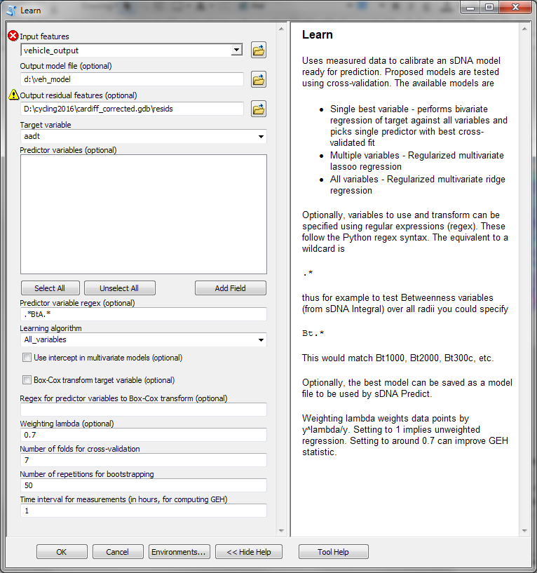
Figure 11: sDNA Learn configuration for calibrating vehicle model.
Inspect the outputs of sDNA Learn. Which variables were used and with what weighting? Is \(r^2\) good enough? If so then jump to step 5.
If \(r^2\) is not good enough, inspect residuals output by sDNA Learn: plot a graph of actual flow against prediction (View → Graphs → Create graph). (These can be selected on the graph to locate them on the map).
Try to figure out where errors come from. They are likely to arise
(a) from network errors; in which case it is worth checking why traffic is not taking the route you expect - perhaps some links are not connected when they should be?
(b) because some behaviour that happens in reality is not accounted for in the model; e.g. flows to town centre or some specific facility, people navigating by means other than most direct route. If desired, run extra models and combine with the existing ones before running sDNA Learn on the outputs of all models together.
See also Troubleshooting Models.
Once you are happy with \(r^2\), use sDNA Predict to predict aadt on the whole network, based on the model file (
d:\veh_model). Note that if your vehicle gates consist of lines rather than points, the variable names must be changed slightly. For example, a variable calledSum_BtA25000on the gates would be calledBtA25000on the network. The model file is a plain text file and can be edited to rename the variables as appropriate.
Calibration is now complete and the AADT field contains traffic predictions for each link in the combined network.
Production of the cycle model
Now that a calibrated estimate of vehicle traffic is present on the entire network, it is possible to produce a cycle model that takes account of vehicle traffic.
If using a unified network, we can now take a copy of only the desired study area plus buffer to account for cycle flows in and out of the area. Most cycle trips are not likely to be more than 4km in length, so this means the study area plus 4km (though a larger distance can be used if desired). Although distances should be measured along the network, it is fine to use simple selection tools and measure these distances as the crow flies – the result will only be that a slightly larger network is used. The actual trip lengths in the simulation are determined by the radius requested of sDNA.
It is worth checking at this point that elevation data has been correctly transferred to the network. One way to do this is to run sDNA Individual Link Measures, with a hybrid metric that captures slope.
Run sDNA Individual Link Measures with analysis type set to HYBRID, and the following advanced config:
linkformula=hg+hlCheck that Hybrid Metric Forward (HmF) in the results from (1) highlights network links which slope.
Run a cycle model. This is again achieved by running sDNA Integral with the analysis type set to CYCLE_ROUNDTRIP. Set the Radial Metric to MATCH_ANALYTICAL: this means the radius is measured as CYCLE_ROUNDTRIP as well.
Choose a variety of radii e.g. 3000, 4000, 5000, 7000, 9000, 12000, 15000, 18000. These are distances in metres adjusted for factors that deter cyclists: slope, traffic and twistiness. Note that CYCLE_ROUNDTRIP uses round trip distances to account for the fact that going downhill is a deterrant if the cyclist must come back up the hill later.
Again, choose Banded Radius.
The sDNA cycle modes are derived from prior research on cyclist behaviour. It is a special case of hybrid analysis. If you inspect the output of sDNA, the equivalent hybrid formula is shown.
Calibration of the cycle model
The cycle model can be calibrated in much the same way as the vehicle one.
If no cycle flow data is available, then an uncalibrated model can be obtained by guessing at which radius of hybrid betweenness to use for the output. The most effective radius from cities similar to the study area would be a reasonable starting point.
If cycle flow data is available, then the best radius is selected using sDNA Learn in the same way as it was for the vehicle models. Having done this, it may or may not be necessary to convert the chosen betweenness variable into a predicted daily flow. The betweenness variable will already show relative levels of flow.
If predicted flows don’t seem to match actual flows, see Troubleshooting Models.
Recommended model outputs
Predicted vehicle flows
These are present on the vehicle network, labelled “aadt” (or whatever you chose to call them during calibration).
Predicted cyclist flows
Uncalibrated flows are available as Betweenness Hybrid for varying maximum trip distances. Calibrated flows will be in a variable of your own creation if the calibration process is followed.
Accessibility
Accessibility is measured by computing network quantity within each distance band. It can thus be measured by the Links, Length or Weight variables, so long as the radial metric is set appropriately (e.g. CYCLE_ROUNDTRIP). If the model is calibrated, you have a few possible approaches
- quick and approximate: run a cycle model without using banded radius. Use sDNA learn in SINGLE_BEST mode to see which single radius best explains cyclist flows, and then measure accessibility for this radius.
- more sophisticated: keep the cycle model based on banded radius. Edit the model file, replacing BtH with Links, Length or Weight as appropriate, then use sDNA Predict to combine accessibility measures across multiple radii in the manner that best explains cyclist flows.
- If mode choice data is available, use sDNA Learn and Predict on the banded cycle model to produce predictions of mode choice. Use predicted mode choice as your definition of accessibility.
Higher numbers show higher quantity of network.
Effect of traffic and slope on accessibility
This is measured by comparing accessibility from the cycle model with an alternative model with no slope or traffic.
First add a numeric field to the network called “zero” and set it to 0 for all links. This is used to simulate zero traffic!
Run a second cycle model as described above but provide the following advanced config: aadt=zero;s=0;pre=no_slope_traffic_
s=0 sets the effect of slope to 0. aadt=zero tells sDNA to use the contents of your “zero” field (which you set to 0) as the traffic estimate.
pre=no_slope_traffic_ changes names for the outputs of the second model for clarity.
Now join the output of this second model back to the original model. Add and compute a data field to work out \(\text{accessibility without traffic and slope}/\text{accessibility with traffic and slope}\). (ArcGIS: computing a field is not necessary. Instead, in the Symbology dialog, select accessibility without traffic/slope as Value and accessibility with traffic/slope as Normalization).
The results are expressed as a ratio, where 1 means traffic and slope have no effect, 2 means traffic and slope make accessibility twice as difficult, etc.
Note that producing flow predictions in the absence of traffic is also possible, and comparing these to flow predictions with traffic can also suggest hotspots to consider for infrastructure improvement.
Effect of traffic on accessibility
As Effect of traffic and slope on accessibility, but use a different advanced config: pre=no_traffic_;aadt=zero
Predicted conflicts
Create a variable that multiples predicted cycle flows by predicted vehicle flows. (ArcGIS: use Add Field and Calculate Field in ArcToolbox - Data Management - Fields). The numbers are an unscaled score indicating relative risk of conflict. Display using only two categories, manually selecting a suitable threshold to identify the links with more conflict potential. The threshold should be set according to need; in terms of identifying incident sites:
- High thresholds increase the rate of both true and false negatives
- Low thresholds increase the rate of both true and false positives
Flows to/from specific facilities
Run a cycle model again, but weighted by the specific facility. This means creating a weight field on the network to denote the facility.
- Add a field named station, hospital, etc
- Set this field to 0 everywhere except for the facility site where it should be set to 1 (ArcGIS: add field, calculate field for 0, then edit the facility itself to set field to 1).
- Run a cycle model with analysis type set to CYCLE_ROUNDTRIP and destination weight set to the field created in (1).
- Display Betweenness Hybrid for the appropriate radius
Accessibility to/from specific facilities
As for Flows to/from specific facilities, but display Mean Hybrid Distance (MHD) for the appropriate radius.
Change to accessibility caused by proposed scheme
This is measured by comparing accessibility as described above, from the current cycle model with an alternative model including the proposed scheme. Run a second cycle model that includes the new scheme and use GIS Spatial Join to bring data from the two models together. It may help to add pre=before_ or pre=after_ to advanced config to label the model outputs differently.
This value can be mapped to show improvement in accessibility, i.e. 1.23 = 23% more destinations to access for the same effort. Alternatively, it can be summed over the entire model to produce a score representing both the increase in accessibility, and the quantity of network that experiences the improvement.
Displaying model outputs
Recommended outputs from the model are discussed below.
We recommend using “graduated colours” symbologies, but modifying the highest bands of any key to display with thicker lines for extra emphasis.
- For flows, we recommend Geometrical Interval classification to give equal emphasis of high and low flows. This is to reflect the fact that flows tend to be exponentially distributed, i.e. most links have little flow but a few links have very high flow.
- It is also possible to display flows using Quantile or Jenks classification. This will condense bands of higher flows and provide more discernment of low level flows.
- For accessibility measures, we recommend Quantile or Jenks classification
- In some cases, e.g. ratios of accessibility, using manual classification may be useful, e.g. to create a special category for ratios equal to 1. A quantile classification can make a useful starting point for a manual one.
In ArcGIS, data on networks is displayed by right-clicking on a layer in the table of contents, → properties → symbology. For any display, click “Classify” from the symbologies dialog to determine how continuous data such as predicted flows is banded into categories.
With larger data sets, ArcGIS will warn that not all data has been sampled to create the classification. This is ill advised as some high-flow links may then fail to display altogether. To ensure all data is sampled, click “Classify” to set a higher number of features to sample.
| [1] | An alternative is to use a hybrid metric for vehicle route choice that includes a random component, so that vehicle routes are distributed between both sides of the carriageway. This may prove useful in cases where one way data is not available. |
| [2] | Note that the DfT release major road and minor road data separately. For effective calibration it is necessary to download both data sets and merge them. |